Maps are defined as polygon, polylines and points defined in cartography coordinates (measured in longitude and latitude). To view such information on a 2D device (such as a screen or printer) you need a way to transform these coordinates to 2D coordinates. In cartography this is transformation is called map projection. It projects geospatial shapes in 2D. Nevron Map for Reporting Services supports 22 distinct projection types. All map layers inside the map use the same projection which is specified by the Projection Type property, that accepts the following values:

	Aitoff - Proposed by David A. Aitoff in 1889, it is the equatorial form of the azimuthal equidistant projection, but stretched into a 2:1 ellipse while halving the longitude from the central meridian.
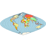	Bonne - a pseudoconical equal-area map projection. All parallels are standard, with the same scale as the central meridian; parallels are concentric circles. No distortion along the reference parallel or the central meridian.
	Cylindrical Equal-Area - represents a cylindrical equal-area projection of the Earth. The following is a summary of cylindrical equal-area projection's special cases: Lambert - standard parallel of 0 degrees Behrmann - standard parallel of 30 degrees Tristan Edwards - standard parallel of 37.383 degrees Peters - standard parallel of 44.138 degrees Gall - standard parallel of 45 degrees Balthasart - standard parallel of 50 degrees
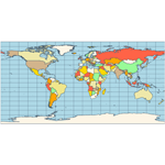	Equirectangular - projection that maps meridians to equally spaced vertical straight lines, and parallels to equally spaced horizontal straight lines.
	Eckert IV - pseudocylindrical and equal area projection. The central meridian is straight, the 180th meridians are semi-circles, other meridians are elliptical. Scale is true along the parallel at 40:30 North and South.
	Eckert VI - pseudocylindrical and equal area projection. The central meridian and all parallels are at right angles, all other meridians are sinusoidal curves. Shape distortion increases at the poles. Scale is correct at standard parallels of 49:16 North and South.
	Hammer - an equal-area map projection, described by Ernst Hammer in 1892. Directly inspired by the Aitoff projection, Hammer suggested the use of the equatorial form of the Lambert azimuthal equal-area projection instead of Aitoff's use of the azimuthal equidistant projection. Visually, the Aitoff and Hammer projections are very similar, but the Hammer has seen more use because of its equal-area property.
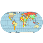
	Kavrayskiy VII - a map projection invented by V. V. Kavrayskiy in 1939 for use as a general purpose pseudocylindrical projection. Like the Robinson projection, it is a compromise intended to produce good quality maps with low distortion overall. It scores well in that respect compared to other popular projections, such as the Winkel Tripel, despite straight, evenly-spaced parallels and a simple formulation. It has been used in the former Soviet Union but is almost unknown in the Western world.
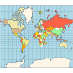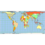
	Mercator - introduced in 1569 by Gerardus Mercator. It is often described as a cylindrical projection, but it must be derived mathematically. The meridians are equally spaced, parallel vertical lines, and the parallels of latitude are parallel, horizontal straight lines, spaced farther and farther apart as their distance from the Equator increases. This projection is widely used for navigation charts, because any straight line on a Mercator-projection map is a line of constant true bearing that enables a navigator to plot a straight-line course. It is less practical for world maps because the scale is distorted; areas farther away from the equator appear disproportionately large. On a Mercator projection, for example, the landmass of Greenland appears to be greater than that of the continent of South America; in actual area, Greenland is smaller than the Arabian Peninsula.
	Miller Cylindrical - a modified Mercator projection, proposed by Osborn Maitland Miller (1897-1979) in 1942. The parallels of latitude are scaled by a factor of 0.8, projected according to Mercator, and then the result is divided by 0.8 to retain scale along the equator.
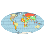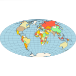
	Mollweide - The Mollweide projection is a pseudocylindrical map projection generally used for global maps of the world (or sky). Also known as the Babinet projection, homolographic projection, or elliptical projection. As its more explicit name Mollweide equal area projection indicates, it sacrifices fidelity to angle and shape in favor of accurate depiction of area. It is used primarily where accurate representation of area takes precedence over shape, for instance small maps depicting global distributions.
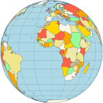	Orthographic - a perspective (or azimuthal) projection, in which the sphere is projected onto a tangent plane. It depicts a hemisphere of the globe as it appears from outer space. The shapes and areas are distorted, particularly near the edges, but distances are preserved along parallels. In NOV Map this projection contains a special property called CentralMeridian, which lets you specify the meridian that should be in the center of the projection (from -90 to 90 degrees). Adjusting this meridian will result in 3D map rotation to the left or to the right, an effect similar to the rotation of a globe.
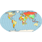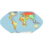
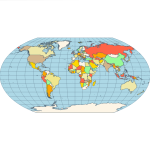
	Robinson - made in 1988 to show the entire world at once. It was specifically created in an attempt to find the good compromise to the problem of readily showing the whole globe as a flat image. The projection is neither equal-area nor conformal, abandoning both for a compromise. The creator felt this produced a better overall view than could be achieved by adhering to either. The meridians curve gently, avoiding extremes, but thereby stretch the poles into long lines instead of leaving them as points. Hence distortion close to the poles is severe but quickly declines to moderate levels moving away from them. The straight parallels imply severe angular distortion at the high latitudes toward the outer edges of the map, a fault inherent in any pseudocylindrical projection.
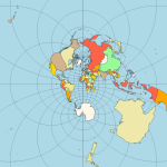	Stereographic - it is a particular mapping (function) that projects a sphere onto a plane. The fact that no map from the sphere to the plane can accurately represent both angles (and thus shapes) and areas is the fundamental problem of cartography. In general, area-preserving map projections are preferred for statistical applications, because they behave well with respect to integration, while angle-preserving (conformal) map projections are preferred for navigation. The stereographic projection falls into the second category.
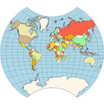	Van der Grinten - neither equal-area nor conformal projection. It projects the entire Earth into a circle, though the polar regions are subject to extreme distortion. The projection offers pleasant balance of shape and scale distortion. Boundary is a circle; all parallels and meridians are circular arcs (spacing of parallels is arbitrary). No distortion along the standard parallel at the equator.
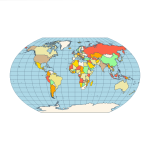
	Wagner VI - a pseudocylindrical whole Earth map projection. Like the Robinson projection, it is a compromise projection, not having any special attributes other than a pleasing, low distortion appearance.
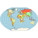	Winkel Tripel - a modified azimuthal map projection proposed by Oswald Winkel in 1921. The projection is the arithmetic mean of the equirectangular projection and the Aitoff projection. Goldberg & Gott show that the Winkel Tripel is arguably the best overall whole-earth map projection known, producing very small distance errors, small combinations of ellipticity and area errors, and the smallest skewness of any map. In 1998, the Winkel Tripel projection replaced the Robinson projection as the standard projection for world maps made by the National Geographic Society.

The View Bounds settings of the map lets you control the part of the map which you want to display. Once the map bounds are determined by the view mode, you can additionally specify zoom percentage and center of the map. Following is a description of properties of the view bounds:

Bounds Mode - defines the mode in which the map bounds are determined. Possible values are:

Fit To Bounds - the map is fitted to automatically determined bounds or custom ones. You can individually specify automatic or custom min and/or max longitude and/or latitude values for the map bounds.

Fit To Layer - the map is fitted to the content of a user specified layer. This is useful when you display multiple layers and want to zoom to a specific one.

Fit to Data Bound Shapes - as explained in the The Map Data Model topic not all records from the map data can be bound to the layer data table due to the nature of the performed Left Outer join. This mode lets you zoom only to the shapes which are bound to data.

Fit to Matching Shapes - lets you fit the map to the shapes that match a specific criteria.

Map Bounds - this settings group is only visible when the Bounds Mode is set to Fit To Bounds. It lets you define the min and max longitude and latitude of the map that is displayed to the user. Each of the four settings (min longitude, max longitude, min latitude and max latitude) can be automatically or manually specified.

Fit To Layer - this setting is only visible when the Bounds Mode is set to Fit To Layer. It lets you select the layer which must be fitted in the view.

Fit To Shape Conditions - lets you specify the conditions which the shapes to which you want to zoom on must match. The shape conditions is a list of items each having the following properties:

Field Name - the name of the field from the joint table from which to get a value for the current shape.

Operator - the operator to use for comparison between the field value and the value of the condition.

Value - the value towards which to compare the value of the field.

Combinator - the way in which the condition is combined with the previous one. If there are multiple conditions the conditions are combined as a sequence of OR groups from AND conditions like this: (C1 AND C2) OR (C3 AND C4). The latter example has AND combinator for condition C1, OR for C2, AND for C3 and the last condition combinator is never used.

The map determines the map bounds that need to be displayed based on the View Bounds settings above. Once these map bounds are determined, the map applies additional zooming and centers the view based on the following properties:

Zoom Percent - defines a zoom percentage with which to additionally zoom the map.

Center Mode - defines the mode in which the map is centered. Possible values are:

Center To Percents - the map is centered to use specified percents relative to the current map bounds.

Center To Layer - the map is centered to a specific map layer.

Center To Data Bound Shapes - as explained in the The Map Data Model topic not all records from the map data can be bound to the layer data table due to the nature of the performed Left Outer join. This mode lets you center the map to the shapes which are bound to data.

Center To Matching Shapes - lets you center the map to the shapes that match a specific criteria.

Center Percent X - defines the X center of the viewport in percentage values when Center Mode is set to Center To Percents. 50 is the X center of the viewport. You can use this property to offset the map horizontally.

Center Percent Y - defines the Y center of the viewport in percentage values when Center Mode is set to Center To Percents. 50 is the Y center of the viewport. You can use this property to offset the map vertically.

Center To Layer - this setting is only visible when the Center Mode is set to Center To Layer. It lets you select the layer which must be centered in the view.

Fit To Shape Conditions - lets you specify the conditions which the shapes to which you want to center on must match. The shape conditions is a list of items each having the following properties:

Field Name - the name of the field from the joint table from which to get a value for the current shape.

Operator - the operator to use for comparison between the field value and the value of the condition.

Value - the value towards which to compare the value of the field.

Combinator - the way in which the condition is combined with the previous one. If there are multiple conditions the conditions are combined as a sequence of OR groups from AND conditions like this: (C1 AND C2) OR (C3 AND C4). The latter example has AND combinator for condition C1, OR for C2, AND for C3 and the last condition combinator is never used.